1. Function Formula ⚓︎
Heart-Shaped Function Formula
where n is a parameter, and the function graph changes as the value of n changes. The domain of the function is: [-1.81, 1.81]
2. Interactive Online Demo ⚓︎
3. Implementation in Excel ⚓︎
3.1 Step-by-Step Guide ⚓︎
- Variable x
- Create a new Excel spreadsheet, and enter
XandYin cellsA1andB1respectively; - Enter
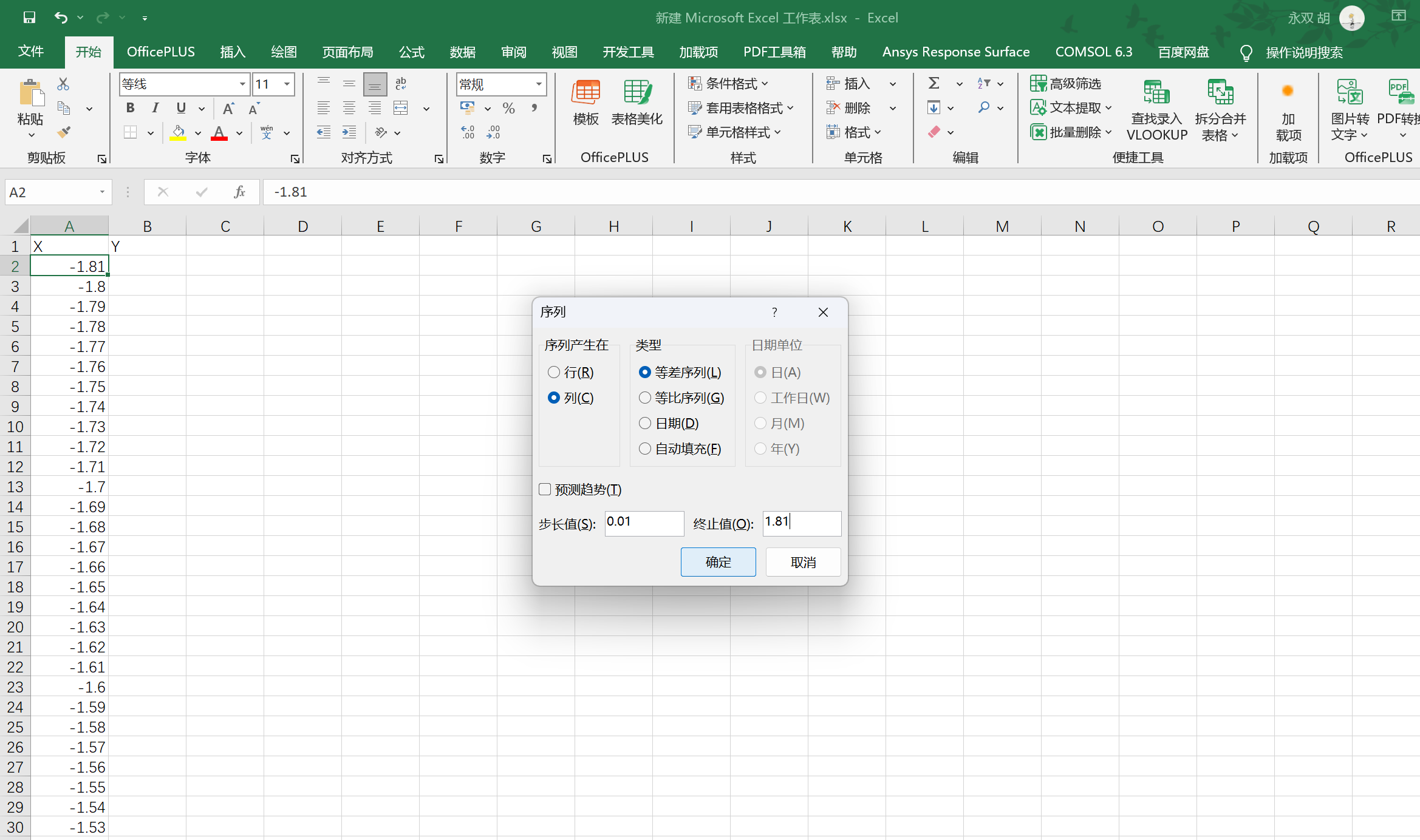
-1.81in cellA2(the left endpoint of the domain); - Select cell
A2, go to theHometab, then findEditing→Fill→Series, open the dialog, select series inColumns, set step value to0.01, and stop value to1.81(the right endpoint of the domain); - This generates all possible values of the variable x for the function in column A.
- Create a new Excel spreadsheet, and enter
- Variable y
- Enter the formula in cell
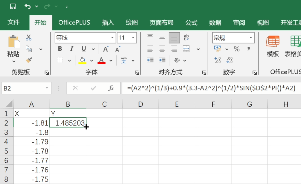
B2:=(A2^2)^(1/3)+0.9*(3.3-A2^2)^(1/2)*SIN($D$2*PI()*A2), where cellD2is the parameter n, and$D$2is an absolute reference (F4 key); - Select cell
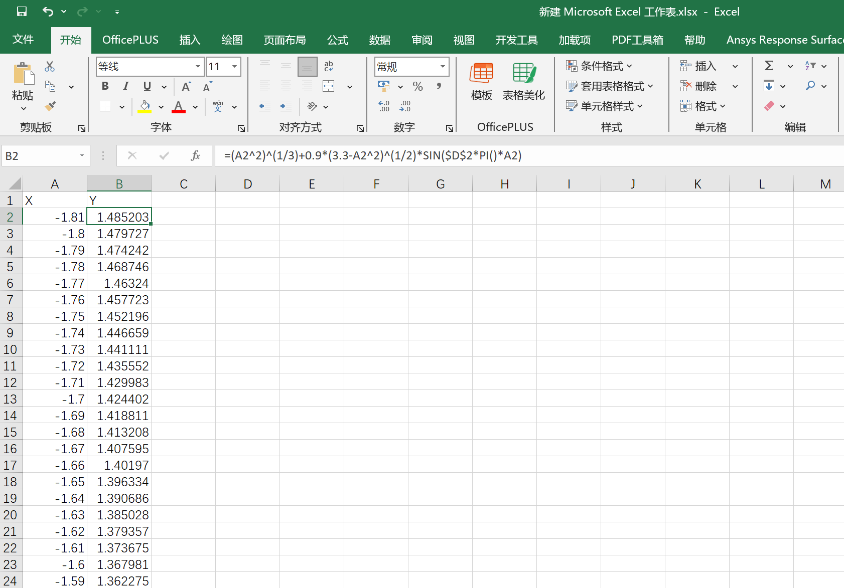
B2, move the mouse to the bottom-right corner of cellB2until the pointer changes to a black cross (fill handle), then double-click the left mouse button to auto-fill the formula downward and calculate the corresponding y values for column A.
- Enter the formula in cell
1 | =(A2^2)^(1/3)+0.9*(3.3-A2^2)^(1/2)*SIN($D$2*PI()*A2) |
- Create the Chart
- Select cell
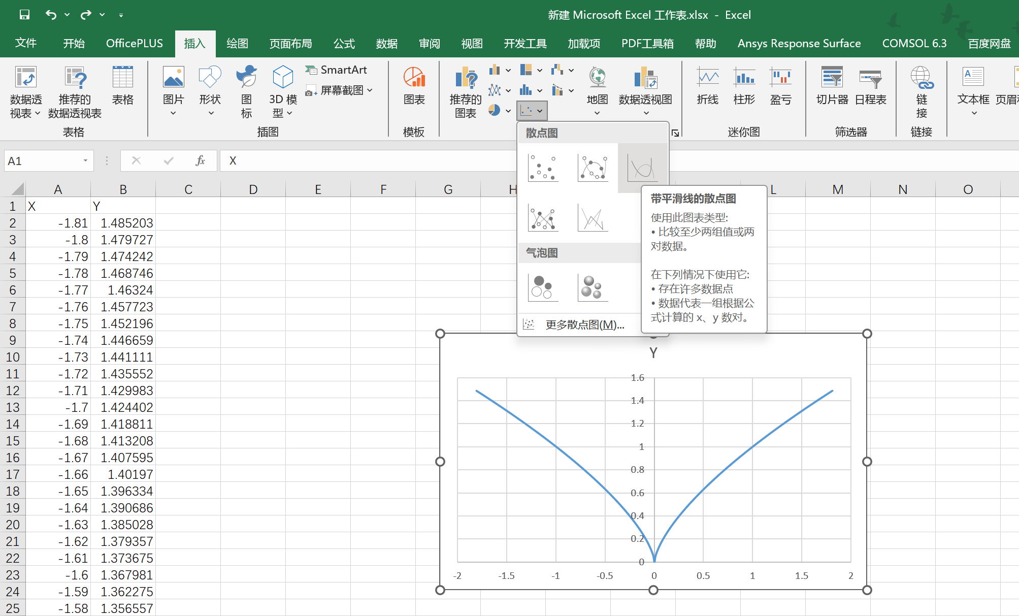
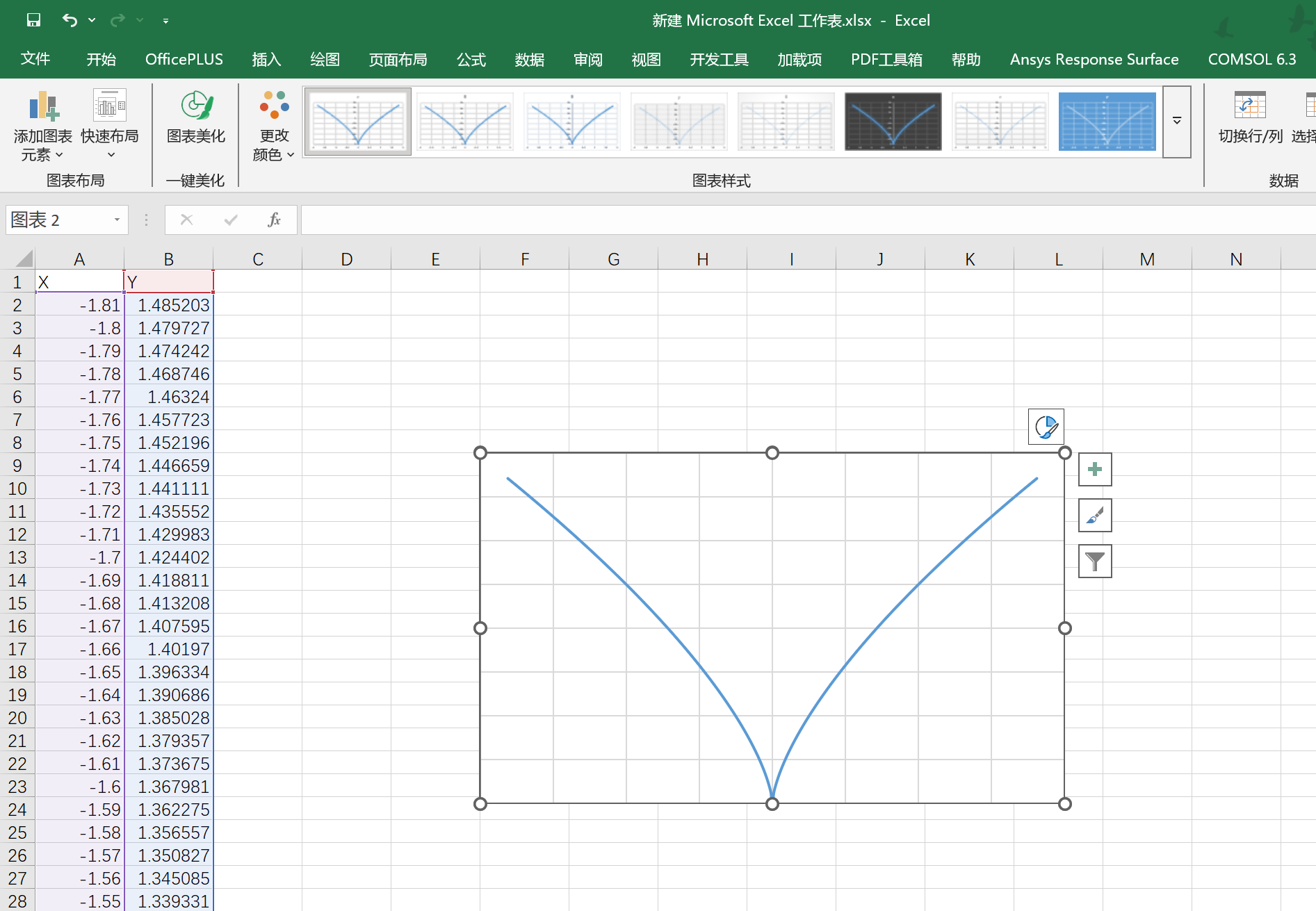
A1, pressCtrl + Shift + →, then pressCtrl + Shift + ↓to select all data in columns A and B; - Go to the
Inserttab, findCharts→Insert Scatter (X, Y) or Bubble Chart→Scatter with Smooth Linesto create a heart-shaped scatter chart; - Click the X-axis in the chart and press
Deleteto remove it; click the Y-axis and pressDeleteto remove it; also delete the chart title and legend.
- Select cell
- Iterative Calculation
- Enter the formula
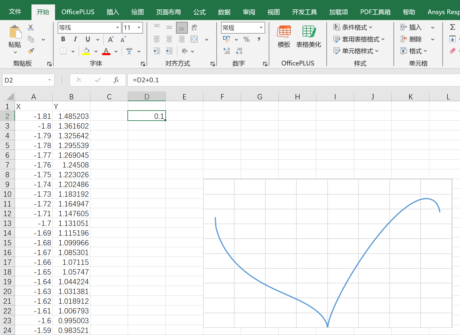
=D2+0.1in cellD2and press Enter; - Select cell
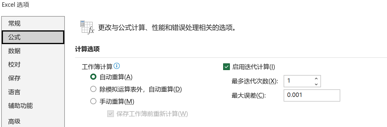
D2, click theFiletab in the top-left corner of Excel, then selectMore→Options→Formulasat the bottom left; - Under the
Calculation optionssection on the right, checkEnable iterative calculation, setMaximum iterationsto1, and clickOKto save the settings; - Hold down the
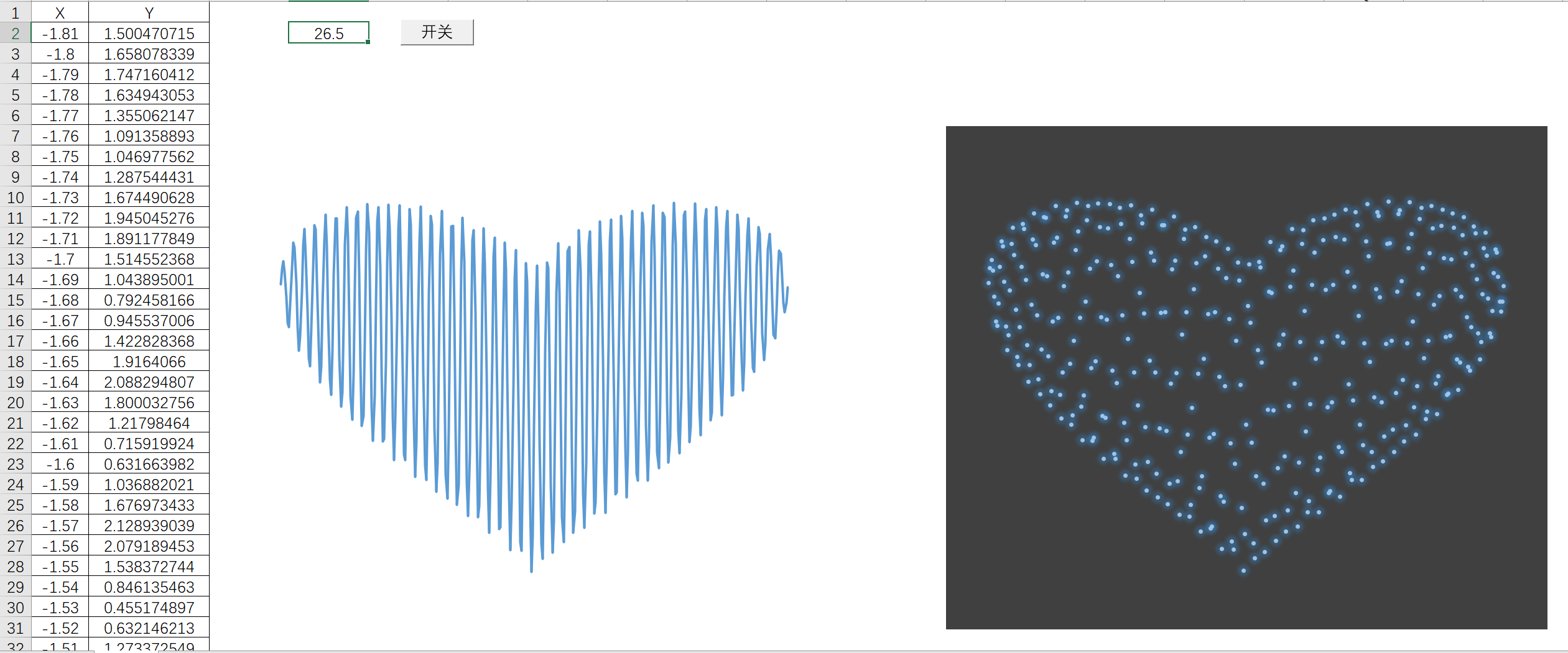
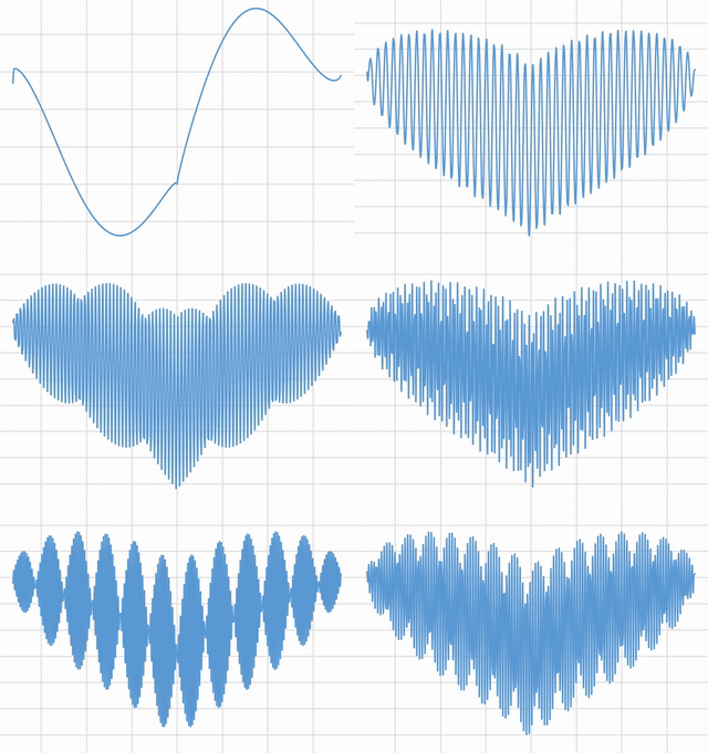
F9key (orFn + F9key) on the keyboard, and the heart-shaped function graph will begin a “beating” animation effect.
- Enter the formula
Result:
3.2 Excel Macro Code for Calculation Control ⚓︎
- Open your Excel file, click the
Filetab in the top-left corner, selectSave As, and set the save type to:Excel Macro-Enabled Workbook (*.xlsm). - Click the
Filetab in the top-left corner, selectMore→Options→Customize Ribbonat the bottom left, checkDeveloperunderCustomize the Ribbonon the right, and clickOKto save.
(1) Form Control: Button ⚓︎
Click Developer, then click Visual Basic, and enter the following code:
1 | Public isLooping As Boolean |
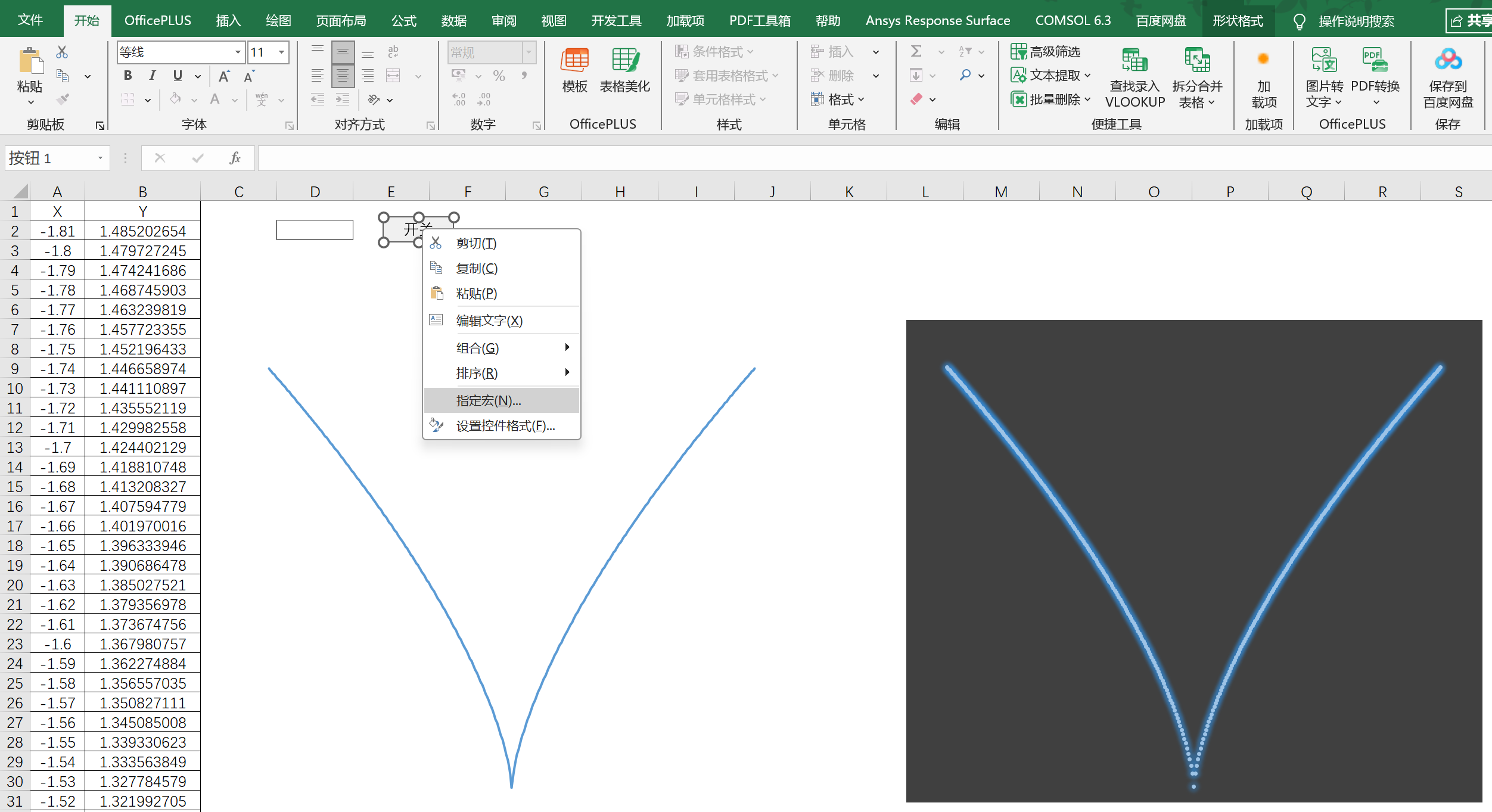
Insert a Form Control: Button, assign the macro 心形图 to it, click OK, and name the button 开关.
(2) Form Control: Start Button and Continuous Toggle ⚓︎
Click Developer, then click Visual Basic, and enter the following code:
1 | Public isLooping As Boolean |
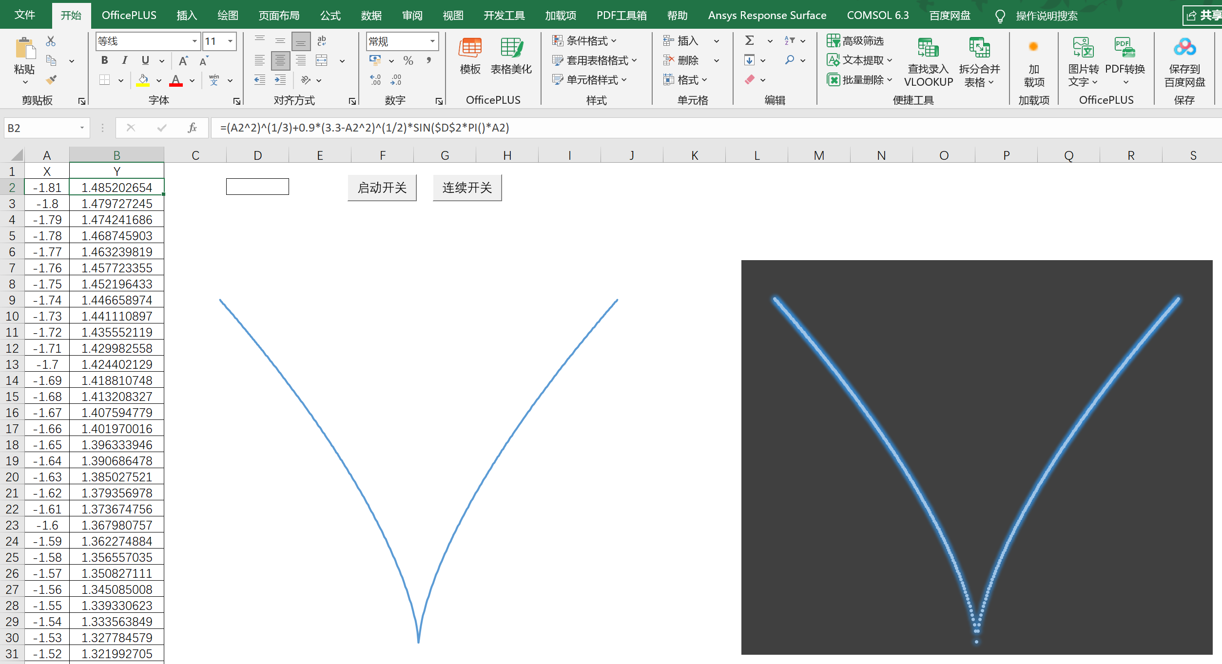
Insert a Form Control: Button, assign the macro 心形图 to it, click OK, and name the button 启动开关 for controlling start/stop;
Insert a Form Control: Button, assign the macro 连续开关 to it, click OK, and name the button 连续开关 for controlling whether parameter n runs continuously.
(3) ActiveX Control: Button ⚓︎
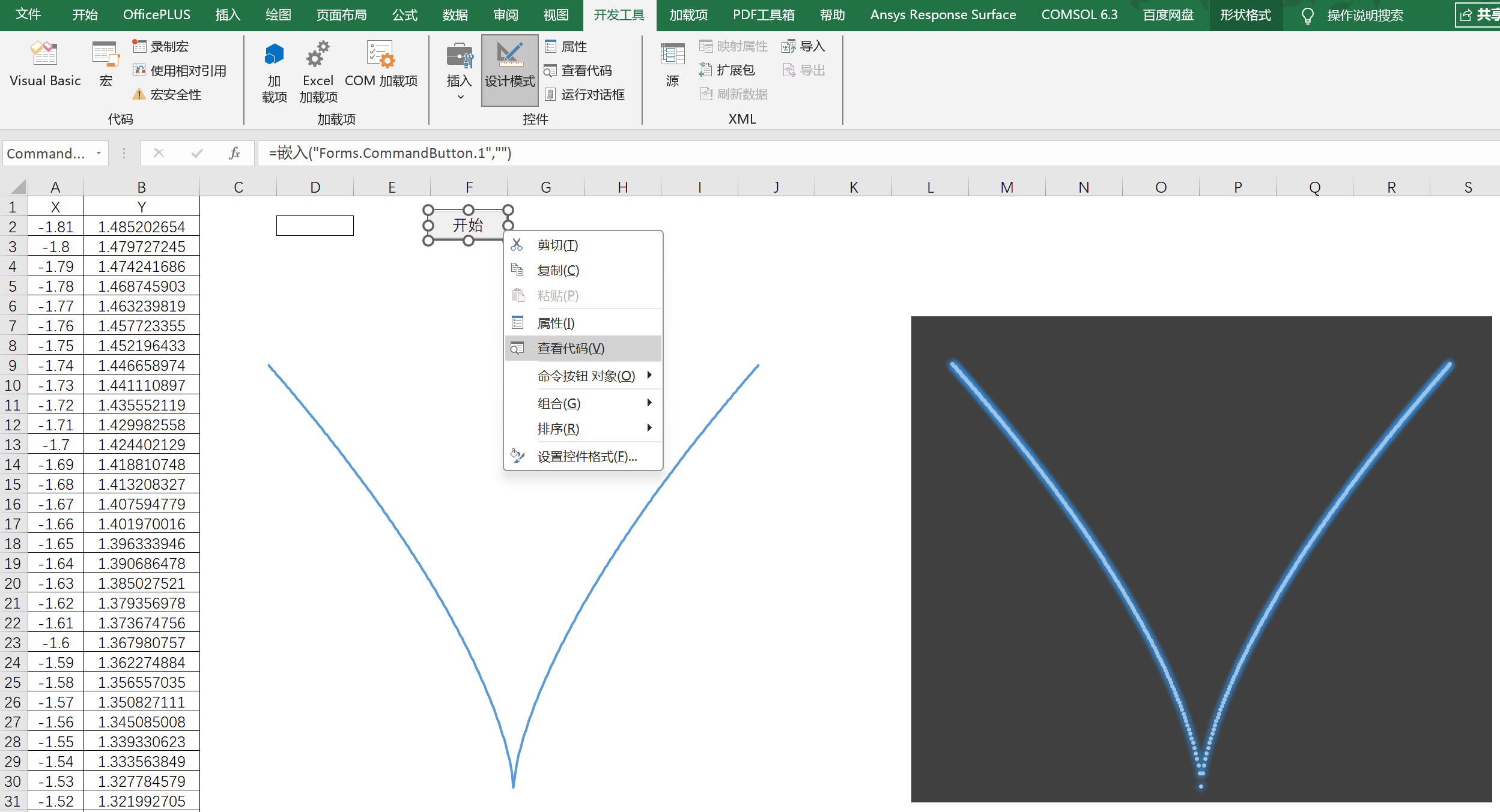
Insert an ActiveX Control: Button, enable Design Mode under the Developer tab, right-click the newly created button, select View Code, and enter the following code:
1 | Public isLooping As Boolean |
(4) Form Control: Scroll Bar ⚓︎
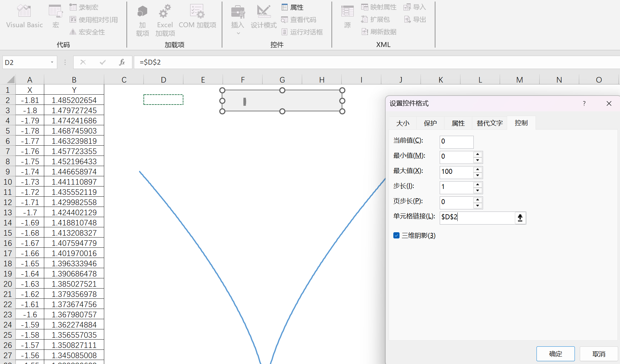
Insert a Form Control: Scroll Bar, right-click the scroll bar, select Format Control, and under the Control tab, set Minimum value: 0, Maximum value: 100, Incremental change: 1, and Cell link: $D$2.
(5) ActiveX Control: Scroll Bar ⚓︎
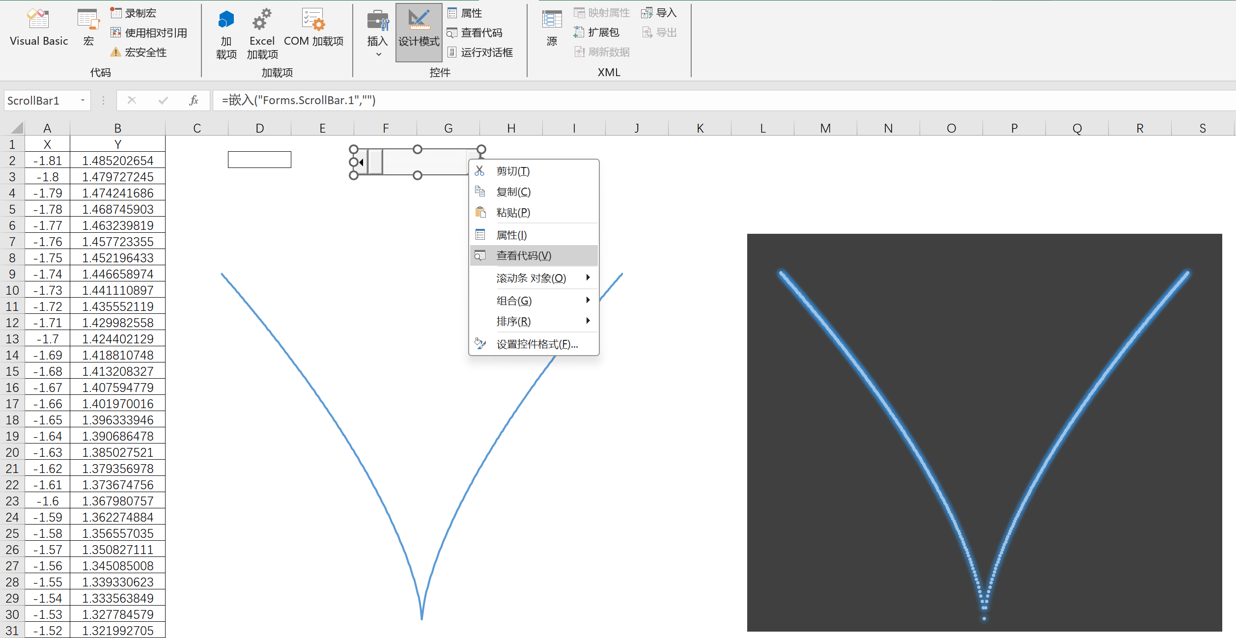
Insert an ActiveX Control: Scroll Bar, enable Design Mode under the Developer tab, right-click the newly created scroll bar, select View Code, and enter the following code:
1 | Private Sub ScrollBar1_Change() |
4. File Download ⚓︎
Click to Download Wechat
 Alipay
Wechat Official Account has more content!